Enhancing Thickness Inspection Efficiency: Data Logging vs. Manual Entry
Application Overview:
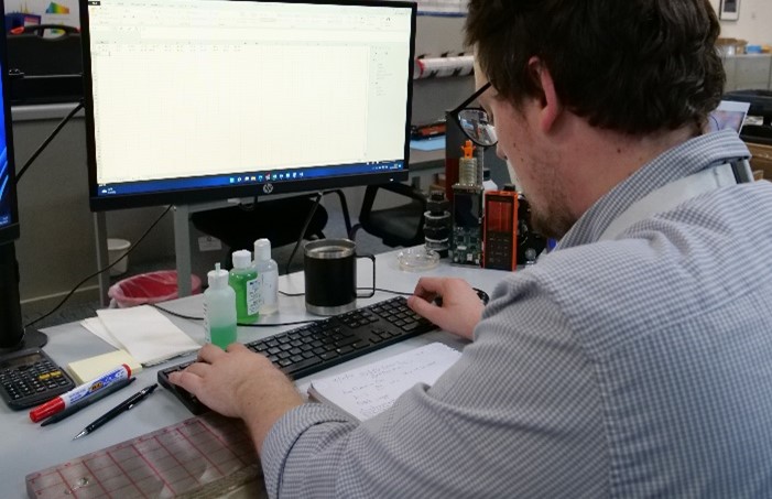
In today’s fast-paced industrial environment, efficiency is key. When it comes to thickness inspection, the traditional method of manually recording measurements in a notebook and then transferring them to a spreadsheet can be time-consuming and prone to errors. However, with the introduction of modern thickness gauges equipped with built-in data-logging capabilities, inspectors now have a more efficient alternative.
This application note aims to compare the time required to complete a thickness inspection using manual data recording versus an integrated data-logging system, using a Dakota CX8-DL ultrasonic thickness gauge. By conducting a controlled experiment and measuring the time taken from the first reading to the final Excel data table, we will quantify the potential time savings achieved by using data-logging thickness gauges over notebooks and pens.
The results of this study will shed light on the benefits of adopting modern inspection tools and techniques, ultimately leading to improved productivity and accuracy in thickness measurement applications.
Experimental Design:
To properly compare these two methods of data collection, it’s important to design an experiment that fairly represents the median case for both. To achieve this, we constructed a simple inspection task to be repeated 3 times for each method to establish an average. We’ve also broken the task down into sections to better understand where the approaches are stronger against each other.
Both tests will start with the plate already marked up into a grid of 25mm x 25mm squares, as the time this takes will be the same regardless of data recording method.
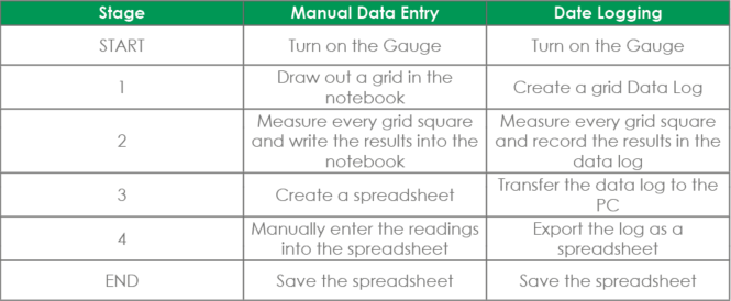
Stage 1: Drawing a Grid vs. Creating a Grid Data Log
In general, if you’re carrying out a grid-based inspection, it makes sense to make a copy of the grid in your notebook to avoid making transcription errors.
We used a grid size of 12x5 (60 readings total) to strike a decent balance of realism and test duration. The gauge we chose for this test, the CX8-DL, has a native grid format when creating logs.

Stage 2: Manual Entry vs. Data Logging
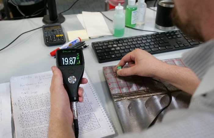
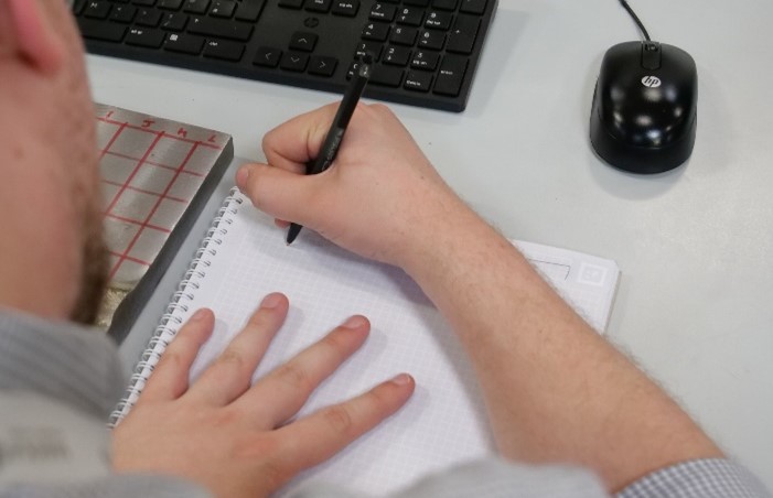
For each square on the Manual Entry tests, the reading is stabilised, observed and then written in the notebook with a pen.
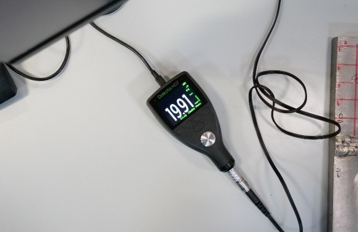
For the data-logging tests, recording each square’s measurement requires simply pressing the ‘Save’ button once the signal has reached 4 or more on the stability bar.
Stage 3: Creating a Spreadsheet vs. Downloading Data Log
It shouldn’t take too long to create a spreadsheet to contain our readings as we simply need to input each reading into the corresponding cell and we won’t be formatting the spreadsheet.
To download a data log we simply need to connect our CX8-DL to a computer with DakMaster installed and follow the log download routine.
Stage 4: Manual Entry vs. Exporting
The final stage for the Manual Entry test is to transfer the measurements from the notebook to the sheet. With practice, this can be accomplished fairly quickly by making use of the numpad, TAB and ENTER.
For the Data-logging test, we’ll simply export the data log as an ‘.xls’ file using the DakMaster export functionality. This can be done more quickly by selecting the ‘Download as Excel’ options, but we’ll be doing it the standard way.
Results
Analysis and conclusions
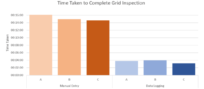
Overall inspection time
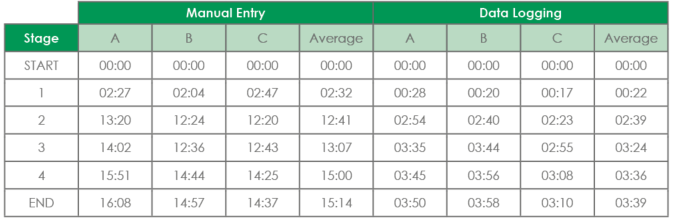
The overall difference in inspection length to take, record and process the 60 grid measurements is substantial, with Manual Entry averaging out to 15:14 start to finish, compared to the Data Logging approach, which came out at 3:39 for the total inspection.
That means for this scenario, choosing to use the digital data logging capacity of the gauge lead to a three quarters reduction in inspection time when compared to manual entry.

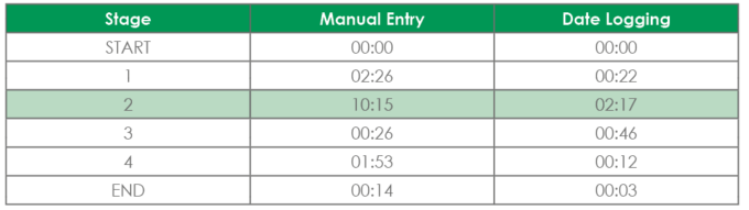
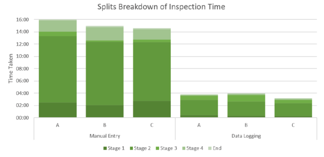
Individual splits
Looking at the individual splits for Manual Entry, the data collection (stage 2) takes the most time by far, followed by drawing out the grid and entering the data by hand. Just drawing the grid took on average 9 seconds longer than it did to perform the entire data collection for the data logging tests.
Comparing Stage 2 for each test, we find a 78% reduction in time from Manual to Digital recording, with the Time per Measurement for Manual Entry sitting at 10.25s compared to Digital’s 2.28s.
Productivity extrapolation
The test inspection area of 240mm x 130mm (9.45” x 5.12”) equates to 0.0312m2 (0.336 sq. ft.) of surface area (approximately 1/30th of 1m2). This allows us to extrapolate a value for ‘inspection time required per m2’ for each method by simply multiplying the mean inspection time by 30, yielding 1hrs 9mins for Data Logging versus 5hrs 8mins for Manual Entry.
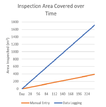
A more useful figure is perhaps ‘inspection area covered per hour’, which works out to:
- 0.857m2/hr for Data Logging (9.23 sq. ft./hr)
- 0.195m2/hr for Manual Entry (2.10 sq. ft./hr)
Assuming a hypothetical inspector works about 8hrs a day, at the 1 year mark, the Data Logging inspector could have measured the entire outside surface of 1.8km (1.12 miles) of a 12” OD pipeline, whereas the Manual Entry inspector will only have managed to measure 410m (0.25 miles).
Transcription errors
One factor that’s also worth mentioning is the possibility for errors in the transcription process. Many studies have been done on the topic of manual data-entry error rates, with the consensus generally coming around the 1-2% error rate for single-entry data transcription. These rates can be significantly reduced with double-entry, but that would obviously nearly double Stage 4’s time cost. Even with doubly-entered data, there’s still a small chance of transcription or omission errors, which are completely eliminated with the data-logging approach.
Dakota gauges used in this application:
For more details on how the Dakota CX Corrosion Thickness Gauge can give an advantage to your inspection process.