How to perform Combined Equipment Test Procedures with Dakota NDT Flaw Detectors
Before any inspection, an ultrasonic NDT inspector needs to ensure that their equipment is working reliably and well to be sure that the results of their inspection are accurate and useful. A good example of these tests and their recommended frequency are detailed in EN 12668-3.
Table 1:
| Test | Frequency | Probe Type |
| Linearity of timebase | Weekly | Both 0° and angle |
| Linearity of equipment gain | Weekly | Either |
| Probe index point | Daily | Angle beam only |
| Beam angle | Daily | Angle beam only |
| Physical state and external aspects | Daily | All |
| Sensitivity and signal-to-noise ratio | Weekly | Both |
| Pulse duration | Weekly | Both |
Typically, these tests are carried out on specially designed calibration blocks, most commonly the V1 and the V2. For the purposes of this application node, we’ll be working with the Metric sized versions, but they’re also available in US-Customary dimensions that align in inches.
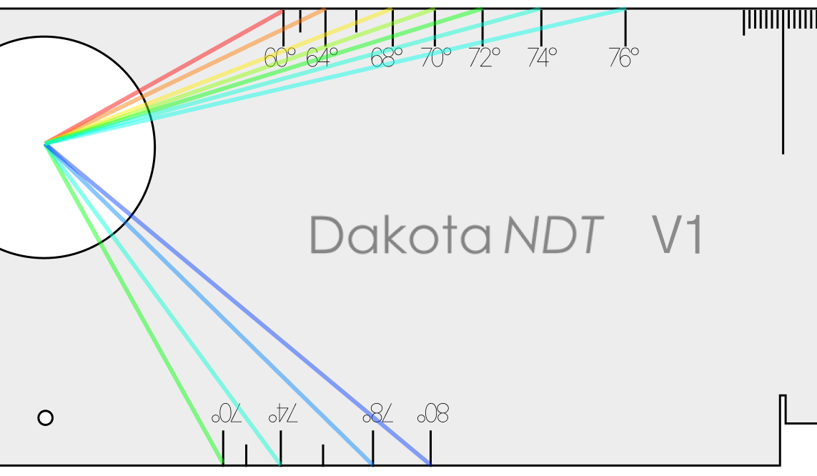
V1 Calibration Block
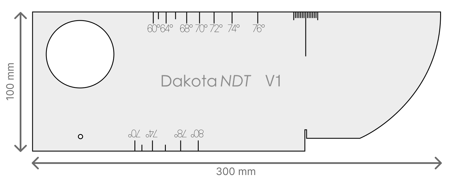

The V1 (also known as the IIW Type 1 or A2) block is the ‘Swiss Army Knife’ of ultrasonic calibration blocks. It allows an operator to test and calibrate multiple important variables necessary to perform a rigorous to-standard manual ultrasonic inspection including beam index point and sensitivity.
It was originally designed in the 1950s for the International Institute of Welding and has remained relatively unchanged since. The construction and dimensions of the V1 block were originally specified in BS 2704 in 1956, but the modern iteration is specified in ISO 2400.
V2 Calibration Block
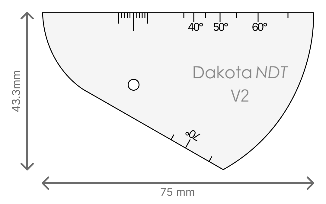

The V2 block, (also known colloquially as the ‘Rompas’ or ‘kidney’ block) is a smaller, more portable alternative to the V1. While it only allows a user to perform a subset of the tests that can be done with the V1, it comes in a much smaller and lighter overall package. (The V2 is typically about 0.4kg / 12oz, compared to the V1’s 5kg / 11lbs.)
It was originally developed in the late 1950s in response to concerns that the V1 could be very difficult to transport for technicians who regularly needed to climb scaffolds and perform inspections in situations with restricted access. The block was first specified in ISO 7963, which was recently updated to be more aligned with ISO 2400.
Technical Note: Digital vs. Analog Verification
Some of the tests these blocks were designed to allow (specifically the linearity tests) were originally designed for analog flaw detectors, where components could drift due to temperature or aging, requiring frequent manual adjustment.
Dakota NDT gauges utilize fully digital signal processing, meaning the "drift" associated with analog CRTs is physically impossible. However, many international standards (ISO, ASME, AWS) still require operators to verify these parameters periodically (e.g., weekly or monthly) to prove the instrument's Analog-to-Digital Converter (ADC) and software are functioning correctly.
Operator Action: Perform these tests strictly according to your specific procedure's frequency requirements.
Gauge Action: If these tests fail on a digital unit, it typically indicates a hardware fault or a need for factory service, rather than a need for manual adjustment.
Time Base Tests
The purpose of this test is to make sure that the gauge’s velocity and zero offset values are set correctly. This is done by testing two different thickness values and using the automatic 2pt calibration routine to align the gauge’s time base with the known material values. There is a technical distinction between calibrating timebase and testing for timebase linearity, but they can be performed at the same time.
Time Base Calibration for 0° Transducers
Suggested Frequency: Weekly
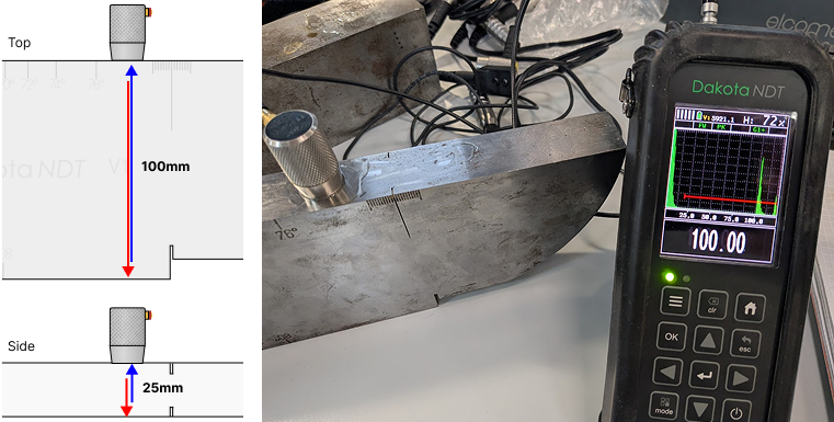
Place your transducer on the side of the V1 block, so that the first gated return echo is from the back wall 25mm away. You first must make sure that the echo signal is visible on screen and currently activating the gate such that a measurement is displayed.
Press the menu button (☰), go to the CAL tab and select MATL 1PT; enter 25.00 when asked to do so.
Move your transducer to the top of the calibration block, in between the index point markers and the angle number engravings. This section is 100mm thick, so we will adjust our gate to start at 90mm.
Once a reading is displayed for this thickness, go back to the CAL tab and select MATL 2PT; enter 100.00 to finalise the calibration.
The gauge will now automatically calculate the material velocity and zero offset based on these two points. Verify the reading is stable.
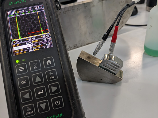
Time Base Calibration for Angle Beam Transducers
Suggested Frequency: Weekly
To calibrate angle-beam transducers we follow a similar procedure, but instead of using the top and sides of the block as our reference points, we instead use the 100mm radiused corner on its first and second echo. We can also use the V2 block, be aware that the intended measurement points are determined by which direction you face the transducer on top of the block.
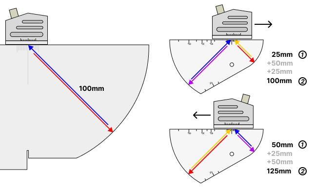
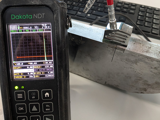
Place your transducer on the index markers pointing towards the curve and adjust it so that the transducer is centred on the block.
‘Peak’ the signal by using minor adjustments to increase the height of the signal to its maximum from that position and then reduce your set’s gain until the 100mm echo is at approximately 80% full screen height.
Once this echo is gated and being measured, press ☰ and navigate to the CAL tab and select MATL 1PT to enter 100.00.
Return to the main screen, adjust the range so that you can see the second echo at 200mm and adjust your gate position so that this echo is targeted, and then perform the same step with the MATL 2PT field but adjusted to 200mm.
Linearity of Time Base
Suggested Frequency: Weekly
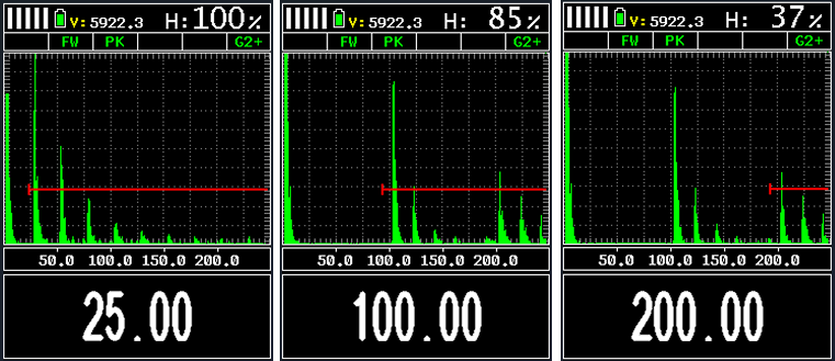
After the previous test, to verify the linearity of the time base, move your gate by adjusting the Gate start point to check each of the repeat echoes from the two positions. You should read each one as a multiple of the first length. I.e. 25.00mm, 50.00mm, 75.00mm. To calculate the error % in linearity, the following equation is used:

To report the linearity, you can record the results and error % in the following table. This example table is given for 0° procedure, for angle beams you should use the 1st, 2nd and 3rd echoes from the 100mm radius.
| First Echo, mm | Second Echo | Third Echo | ||
| Measured, mm | Linearity Error % | Measured, mm | Linearity Error % | |
| 25.00 | 50.03 | 0.012% | 74.94 | 0.024% |
| 100.00 | 200.01 | 0.0004% | 299.97 | 0.009% |
Modern digital flaw detectors are typically able to achieve time base drift of less than ±0.4% across their entire range, but the standards (as written for older analog gauges) will typically say anything less than ±2% is acceptable.
Linearity of Equipment Gain
Suggested Frequency: Weekly
This test verifies that the gain control produces accurate, proportional amplitude changes across its range. Gain linearity is an important component of gain-based sizing methods used extensively in ultrasonic testing to estimate the size of indications within materials.
Position the probe to obtain a signal from a small reflector (small hole on V2 or V1)
Adjust gain to set the signal to 80% FSH - record this as your reference gain value
Increase gain by 2 dB - signal should exceed 100% FSH
Return to reference gain
Decrease gain in 6 dB steps, checking peak amplitude at each step
| Gain Change | Expected FSH | Acceptable Range |
+2 dB | >100% | ≥95% |
0 dB | 80% | (reference) |
−6 dB | 40% | 37–43% |
−12 dB | 20% | 17–23% |
−18 dB | 10% | 8–12% |
−24 dB | 5% | Visible, <8% |
If any reading falls outside the acceptable range, this indicates a gain linearity fault requiring factory service, but this is very unlikely to be an issue on modern digital flaw detectors like the Dakota FX71.
Probe Index Point
Suggested Frequency: Daily
The probe index point refers to the specific location on the transducer shoe that the ultrasonic pulse transmits from. It’s important to calculate this point precisely to ensure that the recorded positions of indications are correct. An accurate index point is also necessary for measuring the true beam angle in a later test.
This test works by using the index markers on top side of the V1 or V2 block and requires ‘peaking’ the signal.
Enable peak hold mode (also known as envelope); press the mode button on the bottom left of the keypad and select PEAK. This will enable an overlay that holds the highest amplitude peak within a region.
Line the transducer up parallel to the block and move the transducer backwards and forwards slowly until you’ve built the full envelope around the peak.
Adjust the transducer’s position to move the active echo signal to the absolute centre of the envelope, when amplitude is at maximum.
The position indicated by the central line of the index marker is your transducer’s index point. Note: Some inspectors mark this position with a pen mark and cover it with clear nail polish to ensure it isn’t washed away through contact with couplant.
Index Point X-Offset
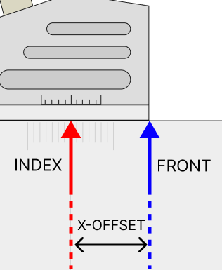
In the TRIG controls within the Dakota FX71 & 81 Flaw Detectors, there is a setting called X-OFFSET; this allows you to adjust the position of the index point in software, so that measurements of position may be taken from the front of the transducer instead of the middle.
To set X-OFFSET correctly, once you’ve established your Index Point, measure the distance from index to front and enter that into the field. Now all along-the-top distance measurements will be shifted to allow measurement from the very front of the transducer.
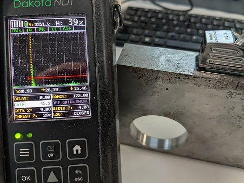
Beam Angle Verification
Suggested Frequency: Daily
The purpose of this test is to verify the angle that the ultrasonic pulse leaves the transducer. While angle beam transducers are manufactured to produce a shear wave that transmits as close to the specified angle as possible, variance in the manufacturing process and wear on the transducer shoe can alter this angle over the lifespan of the transducer. This variance means it’s very important for inspectors to be able to measure the true angle of the beam, to ensure correct location of found indications.
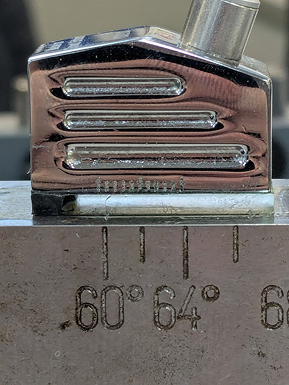
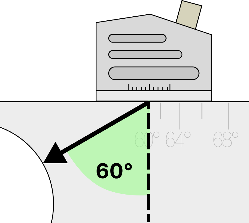
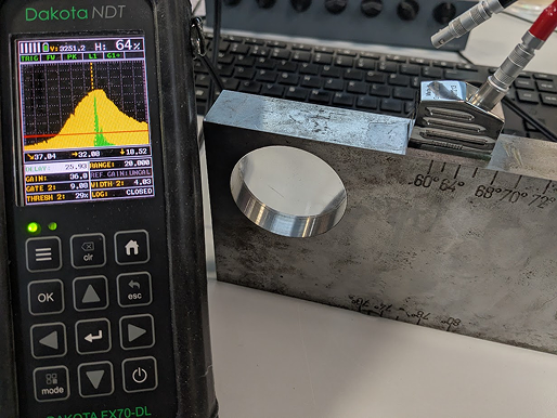
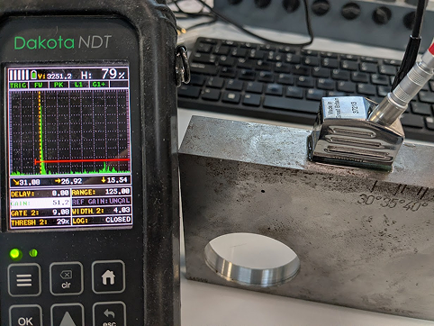
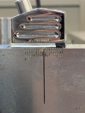
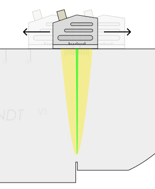
Chose the closest angle to your transducer’s specified angle and place it facing towards the Perspex circle on in the corner of the block. The angle markers are placed so that the closest path between them and the centre of the circle is at the specified angle, i.e. the line from the 60° marker is at exactly 60° from straight-down, facing the circle.
Using the same ‘peak’ technique as for the index point, slowly move your transducer back and forth across the block until you’ve maximised the peak height within the envelope.
Record the position on the scale where the reflected echo is at its maximum size; this is the true beam angle and is indicated by where the index point meets the scale. In the picture above, the beam angle of the transducer is 62°.
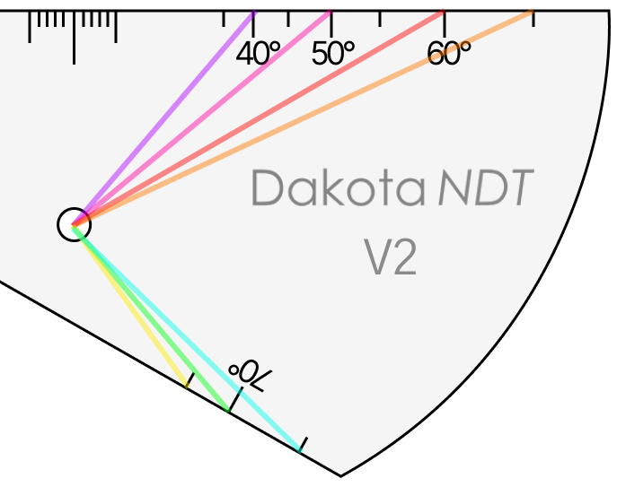
The test is identical for the V2 block, with the only difference being that the target to maximise the echo height of is the small side drilled hole.
Physical State and External Aspects
Suggested Frequency: Daily
This is the simplest of the checks but arguably the most important as a damaged probe or cable can make inspection impossible or interrupt a high-priority shutdown workflow to replace equipment.
Transducer:
Shoe/face for scratches, chips, pitting, or uneven wear
Wedge (if angle beam) for cracks or separation from the crystal housing
Cable connector for bent pins or loose fit
If the transducer is a quick-change shear wave with wedge, make sure to top up the couplant reservoir in the wedge.
Cable:
Outer sheath for cuts, kinks, or crushing damage
Connectors at both ends for damage or intermittent connection (wiggle test while watching for signal dropout
Gauge:
Display for dead pixels or damage that could obscure readings
Keypad/controls for stuck or unresponsive buttons
Connectors for physical damage
Battery level is suitable to get through the full shift, or replacements are to-hand.
Calibration Blocks:
Check surfaces for corrosion, scratches, or contamination that could affect coupling
Ensure any inserts (e.g. Perspex circle in V1) are present and undamaged
If any damage is found that could influence measurement accuracy or reliability, the affected component should be replaced or repaired before inspection work continues.
Sensitivity and Signal-to-Noise Ratio
Suggested Frequency: Weekly
This test monitors the combined sensitivity of the transducer, cable and gauge as a complete system. When the set is first used, a baseline value needs to be established that is then compared against the results of repeated weekly tests to detect sensitivity degradation.
Position the transducer on the calibration block in the same position as the gain linearity test (targeting the side-drilled hole on the V1 or V2 block)
Peak the signal to maximise its amplitude and then adjust the gain to set the signal to 20% FSH; the value in GAIN is your sensitivity value.
Change the position and width of the gate to bracket just the currently acquired SDH echo.
Remove the transducer from the block and clean off any remaining couplant on its face, leaving it uncoupled next to the block (in free air).
Increase the gain until the noise floor grows to begin triggering the gate; record this second gain value as your noise value.
Calculate Signal-to-Noise Ratio using the following formula: Signal-to-Noise Ratio = (Noise Value) - (Sensitivity Value) in dB
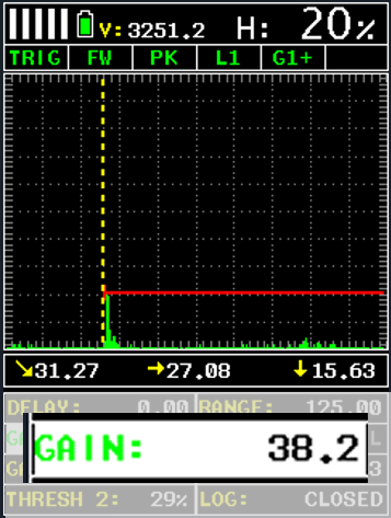
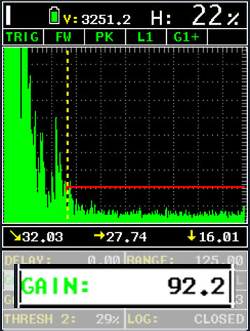
For this example, our SNR = (92.2) – (38.2) = 54dB.
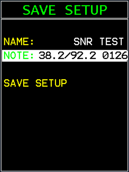
Note: To ensure a fair test against the original baseline values, we recommend creating a setup file for sensitivity checks after the first one is completed to ensure that no accidental changes cause inconsistent results later.
Both the sensitivity value and the signal-to-noise ratio “shall be within ±6dB of the established baseline values” (EN 12668-3: 3.4.3.3). We recommend recording these values in a weekly logbook kept with the equipment.
Note: A drift beyond 6dB should be investigated to ensure no components have become damaged; it’s significantly more likely to be a transducer or cable issue than a gauge one.
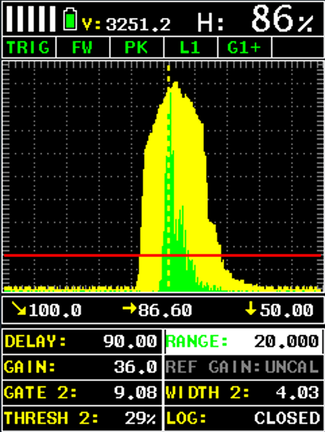
Pulse Duration
Suggested Frequency: Weekly
This test checks that the overall pulse shape hasn’t degraded, which could indicate issues such as degraded transducer damping or gauge amplifier faults. As with the sensitivity tests above, pulse duration is established as a baseline for the full set of equipment and is checked for degradation that might indicate a replacement or repair is needed.
Place your transducer on the index position of the V1 block and obtain a reading from the 100mm radiused section.
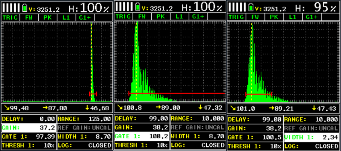
Adjust the gain to set the signal height to exactly 100% FSH
Set the gate threshold to 10% and then move the start of the gate until it touches the waveform.
Reduce the gate’s width until the back of the gate touches the other side of the waveform.
Record this width value as your pulse duration in mm in a logbook with the equipment to allow for later comparisons.
According to EN 12668-3, the pulse duration “shall not exceed 1.5x the baseline measurement”, which means for our example below, the equipment should be checked, or components should be replaced, if the pulse duration ever increases from 2.34mm to 3.51mm.
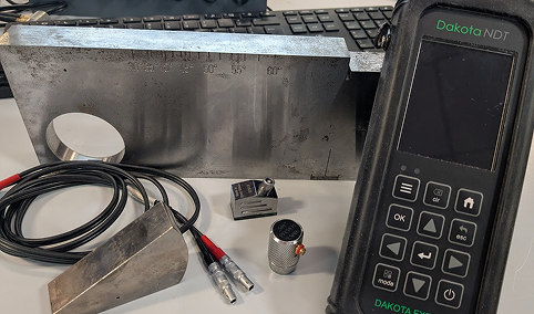
Dakota gauges used in this application:
Dakota FX71-DL Flaw Detector
For more details on how the Dakota FX71-DL Flaw Detector can give an advantage to your inspection process.